Land Degradation - Background

Anthropogenic land degradation

 

 

Placing land degradation in the context of ecological processes

 

 

Principal Investigator:  Dr. Steve Prince

Department of Geographical Sciences, University of Maryland, College Park, MD, USA    sprince@umd.edu

 

 

 

Land degradation is globally pervasive and, in some places, irreversible.  Humans have historically modified the environment directly and indirectly to meet their requirements, but the rate and extent of degradation has accelerated dramatically in recent years. The resulting anthropogenic impacts on land have been so profound that a new geologic era has been recognized, the Anthropocene - generally dated from 1950.

 

The process and state of degradation is well-recognized, and even addressed by a United Nations agency - the UN Convention to Combat Desertification (UNCCD), to which almost 200 nations are signatories.

 

Many studies have contributed to the current theoretical understanding of land degradation. However, some critical aspects that underlie existing knowledge remain to be addressed. Even in the context of extensive study, surprisingly, there remain serious gaps is in the basic foundation of understanding. Clearly, a foundation should contribute to the extensive existing progress to build a coherent whole, rather than proposing yet another conceptual framework.

 

What is “degradation” in the ecological context?

 

 

There is a distinction between, on the one hand, the human causes, motivations and consequences of land degradation and, on the other, the biophysically imposed constraints. This relationship was first developed by Carl Saur and has long been recognized in geography under the title "possibilism" (Robbins, 2012).The term “biophysical” is used here to distinguish the human from the ecological perspectives, although humans are inextricably associated with the ecological.

 

It is important to recognize that environmental processes alone, can result in conditions that take the form of anthropogenic degradation (such as natural hillslope erosion), but are not anthropogenic drivers of “degradation” per se, unless the natural process is initiated or exacerbated by humans (such as erosion following removal of vegetation).

 

Degradation results from a multitude of drivers and can manifest in many forms, including erosion, loss of carbon stocks, and changes in hydrological regimes. It can be driven by changes in land cover, caused by, for example, pollution, pests and diseases spreading as a result of climate change, excessive livestock production, agriculture, forestry, alien species introductions, abandonment of land, mining and urbanization. Thus “degradation” is not a single phenomenon - the term encompasses a wide range of causes and conditions that reduce ecosystem services (Millennium Ecosystem Assessment, 2005).

 

History of degradation studies

 

Land degradation predates modern written history. For instance, an early well documented example is from 2,400 BC in Mesopotamia, where irrigated agriculture in the Tigris and Euphrates valleys led to salinization (Thomas & Middleton, 1994). Notwithstanding this long history, modern day attempts to quantify the extent and scale of land degradation have proven difficult, especially at the global scale.

 

There has been a failure to agree on what ecosystem conditions should be regarded as degraded, hampering any consensus on location, severity and extent. In forested areas, there is extensive mapping of forest loss (i.e., the transformation of forests to other land type), but there are far fewer data on the extent of degradation within untransformed forest.

 

Early global assessments of degradation had a narrow soil focus (e.g., Oldeman, Hakkeling, & Sombroek (1991) but more recently studies have been based on loss of net primary production, often using satellite data (Jackson & Prince, 2016; Noojipady et al., 2015; Prince, 2016; Prince et al., 2009). Following from the Millennium Ecosystem Assessment (Hassan et al., 2005), the emphasis has been on declines in the flow of ecosystem services. Assessment methods have ranged from estimation by specialists; detailed analysis of satellite observation products; social assessment of abandoned land; and simulation models (Prince, 2016; Wessels et al., 2008, 2012).

 

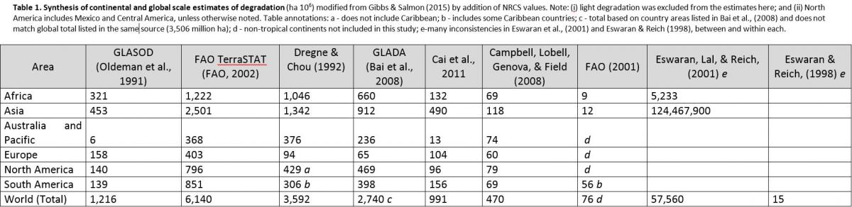
Comments such as 80% of the global croplands are degraded, or that 10-20% of rangeland are degraded are common and often cited (Adeel, Safriel, Niemeijer, & White, 2005; Gibbs & Salmon, 2015), however, progress towards a credible measure of the extent of land degradation remains elusive. The GLASOD “World Atlas of Desertification” (Oldeman et al., 1991) has been widely used, but recent reviews (Prince, 2016; Sonneveld & Dent, 2009) have found it to be seriously faulted to the point it should not be used (Sonneveld & Dent, 2009). Although a number of other attempts have been made at quantifying the global extent of degradation (Table 1) (Gibbs & Salmon, 2015), at the global scale, the spatial locations and severity of degradation remain substantially unknown (Prince, 2016). The 3^rdedition of the World Atlas on Desertification has taken the position of not attempting to develop a single degradation map, but rather uses a convergence of evidence approach (Cherlet et al., 2015).

The degradation process

 

As noted above, there has been and continues to be confusion over the meaning of the term “degradation”. Many believe they can recognize it when they see it (in the field or with satellite imagery), yet the confusion in the literature belies this view. The definition of the term has led to interminable reviews (see review by Vogt et al., 2011) and even comprehensive versions often give rise to confusion.

 

The analogy of a cusp threshold (Figure 1) illustrates the distinctions between some of the different types of degradation. The effects of stress caused by human activities to which organisms are susceptible, and therefore the ecosystem service they provide (e.g., depleted soil nitrogen and crop production), can be envisaged as a “response curve”. This is shown by the blue curve from 1 to 2 to 3 (Figure 1). The ecosystem service responds rapidly, almost linearly (from point 1 to2), until the stress declines (e.g., nitrogen is added in the crop example). As the stress declines from left to right in Figure 1, further increases in the service (crop yield) decrease (from 2 to 3), often reaching a plateau when additional reductions of the specific stress have no further effect (at 3). Fluctuations in the stress cause the ecosystem service to move up and down the curve in its range of resilience (2). On the other hand, there are conditions in which stress drives down the provision of the service, as illustrated by curve 4, until it reaches a threshold (point 5) (Turnbull et al., 2008) at which the ecosystem service drops dramatically. This is an example of a non-linear ecological process. Most importantly the ecosystem service cannot be recovered no matter how much the stress is relieved. In this level of degradation, shown as the lower part of the red curve, the ecosystem reaches its completely degraded condition (point 6): this is the permanently degraded condition described in Vogt et al., (2011).

 

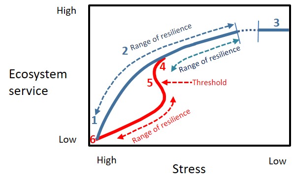
Figure 1 Two types of response to stress. In curve 1, 2 to 3 (blue) the degree of anthropogenic stress determines the level of ecosystem service over the full range, until point 3 when the stress is so low that it has no further effect. The second curve (4 to 6) reaches a threshold (5) at which the response to stress is non-linear and changes to a new state that cannot return to the upper level, no matter how much the stress is alleviated. Illustration based on Lockwood & Lockwood (1993). 

 

The analogy of response curves is helpful only when one anthropogenic stress is involved, but normally there are many that affect ecosystem services, such as: soil type, pollution, soil compaction, loss of palatable species for livestock, reduced productivity. These stresses can be divided into two classes (Figure 2): the first are those that are caused by the physical environment with no human involvement and the second, those that are brought about by human action alone (anthropogenic stresses). These two classes of stress frequently occur together and interact.

 

While a service may be resilient to the full range of anthropogenic stress when there is negligible environmental stress, a moderate environmental stress moves the anthropogenic response curve closer to the threshold (Figure 1). A further increase in environmental stress drives the site over the cusp and into the zone of permanent degradation, from which no return is possible without drastic, expensive and lengthy artificial remediation. Typically neither anthropogenic nor environmental stress alone drive the site into the permanently degraded zone, but when they work together catastrophic loss of services can ensue.

 

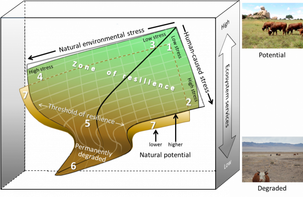
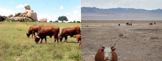
Figure 2 Conceptual representation of the states and process of degradation and the potential contributions of anthropogenic (human-caused) and natural environmental stresses. The ecosystem service(s) is represented by the vertical dimension and the ecosystem dynamics by the surface. The higher up the surface in the vertical dimension, the higher the ecosystem service. The top two edges represent stress from the natural environmental (left) and anthropogenic stress (right). Both stresses increase across the surface (from 1 to 2 and from 3 to 4). The fold in the surface (at 5) represents the threshold of a zone of permanent degradation. Sites that move over the threshold of resilience on any trajectory cannot return to the upper zone of resilience. A second surface shown below (7) represents a site that naturally provides lower environmental services, but is not initially degraded: it has all the features of the upper surface including resilience and the possibility of permanent degradation.

 

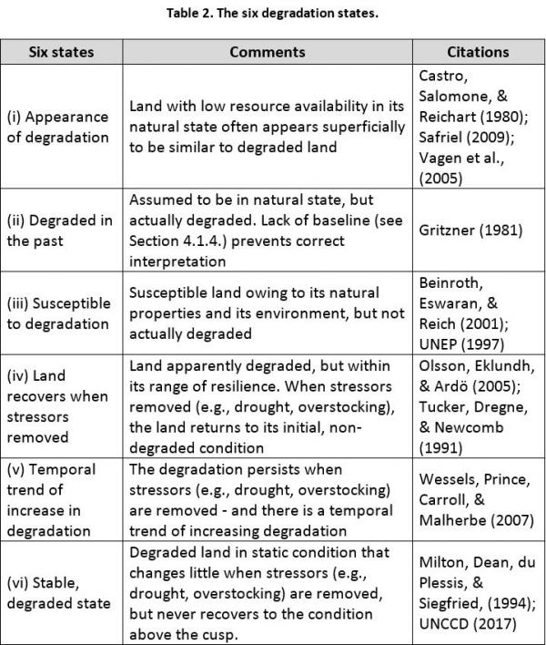
These concepts lead to recognition of six types of “degradation” (Table 1) (Prince, 2016). Types i and iii are actually not degraded, but are often mistaken for it. Recognition of this distinction can be difficult, but it is critical when assessing the status and planning for restoration – the initial failure to recognize these two states and their difference from true degradation has caused much confusion, for example understanding of Sahelian “desertification” (Herrmann & Sop, 2016). A lot of “degradation” mapping is actually about measuring differences in potential of the ecosystem to provide services, not degradation of that potential (Vagen et al., 2005). Similarly Type ii may have existed for a long time and might be assumed to not be degraded, but it could belong to Type vi (i.e., permanently degraded). Types v and vi are the only states that deserves the term “degradation” (Adeel et al., 2005; Vogt et al., 2011), since their condition is effectively irreversible, even when the driver of the stress is removed. The degradation below the threshold is generally not static, but also moves according to its resilience as the stress varies (Type v) (Wessels et al., 2007), but never back over the threshold. Completely static degradation (Type vi) does occur, for example in heavily salinized cropland. Type iv is of greatest interest since, if the stress is alleviated, it has the capacity to recover naturally – although recovery may be accelerated by human intervention; the alternative being unremitting further degradation to Type v or vi.

 

Recovery from Types v and vi is actually possible, but only with significant efforts and expenses, or over exceptionally long-time periods, generally exceeding a human life-span. Moreover, the value of the restored land rarely merits the cost of restoration/recovery. For example, the 20 million ha of the southern Great Plains of the USA that were lost to the “Dust Bowl” in the early 1930s (Baveye et al., 2011; Hurt, 1986; The Nature Conservancy, 2016) were restored at the cost of approximately $17 billion (in 2017 US$) and the creation of an entirely new government agency (now called the Natural Resource Conservation Service) in 2017 employing 12,000 people in 2,900 offices. Nevertheless, land in Type vi remains low and susceptible to renewed degradation (Romm, 2011).

 

 

Remediation and restoration techniques are frequently applied to control degradation. However, the recovery of the original, pre-degradation ecosystem is at best extremely slow. In cases where there are data, disturbance remained detectable over long periods. For example, after 80 years sites in the USA shortgrass steppe, still show the degradation caused by grazing and burning (Peters et al., 2008) - there is no evidence of complete recovery. many such cases have been recognised, a common one being soil compression by heavy vehicles (Webb, 2002). Thus degradation can be permanent on century-long scales. In the ecological literature, this state is referred to as a deflected succession, a subclimax, or plagioclimax.

 

Detection of degradation

Types of data used for mapping large areas

 

Developing indicators and monitoring them are essential to any understanding of land degradation. In the report “Ecological Indicators for the Nation” the National Research Council (2000) provides criteria for selection of indicators, including methods for integrating complex ecological information into multimetric indicators, that can summarize ecological conditions and processes. Anthropogenic land degradation generally consists of multiple conditions and so most monitoring programs use several indicators (Lorenz & Lal, 2016; National Research Council, 2000). The Sustainable Development Goal Target 15.3 has proposed three indices (CBD, 2016), UNCCD uses 11 (Berry et al., 2009), WOCAT uses 57 (Liniger et al., 2008), and GLADA uses 132 (Nachtergaele & Licona-Manzur, 2008).

 

Data on land degradation that are appropriate for rigorous analysis and development of policy-relevant conclusions are the same as those that apply to all quantitative data collection. They have little meaning unless accompanied with explicit information on the methods used, any necessary qualifications and the variance of the reported values. For example, much of the information on the carbon cycle (Lorenz & Lal, 2016) has confidence limits. Qualitative data (including as indigenous and local knowledge) can also have error metrics and can be combined with quantitative data and statistical methods for example in joint analyses, known as “mixed methods” (Creswell, 2007). Data are collected at a wide range of spatial and temporal scales - from single points or small areas of a few hectares, all the way to global, and for one point in time to monitoring long-term trends.

 

Methods differ for different scales. Global measurements are almost entirely made using remote sensing since they can have global coverage, spatial resolutions of a few meters and daily, monthly and annual repeat measurements. In the case of vegetation, the remarkable characteristics of remotely-sensed measurements of vegetation indices (especially normalized difference vegetation index) and their inter-annual trends are compelling.

 

However, while no trend, or no trend after environmental normalization (Bai et al., 2008; Rishmawi et al., 2016), suggests no degradation, that is true only for Type i. (Table 1); the same lack of trend occurs for Type ii. (degraded in the past) and for Type vi. (stable permanently degraded state) - the worst form of degradation.

 

Another issue is that, while the normalized difference vegetation index is a surrogate for vegetation production (gross primary production) it is only a proxy, and can be incorrect in some conditions (Prince, 1991). Other information, such as plant diversity, generally cannot be measured directly. Some interspecific differences can be detected in repeat observations throughout the season based on seasonal phenological changes in normalized difference vegetation index. More direct detection of species has been achieved in some cases using many more spectral bands, but the “spectral diversity” often consists of more than one taxonomic species (Gholizadeh et al., 2018).

 

Degradation generally extends over long time scales - “long-term”, “permanent”, yet there are frequent attempts to account for the long-term at the scale of factors such as annual stocking rates, whereas soil formation has a time scale of many years. Both processes are relevant to degradation, but in quite distinct ways related to their scale of action (Jeltsch, Milton, Dean, & Van Rooyen, 1997; Weber, Moloney, & Jeltsch, 2000; Wiegand, Saitz, & Ward, 2006; Wiegand & Milton, 1996; Wiegand, Milton, & Wissel, 1995). Further, many areas of current degradation, degraded prior to current satellite-based trend data and hence may appear as stable land in these data sets (Gibbs & Salmon, 2015). The same occurs over space, for example deposition of wind-blown products of surface erosion can takes place over hundreds of square kilometers, and hundreds of kilometers from the source, yet cattle hoofs that compact the soil are limited to paddocks measuring hectares. The scale of national politics is another range of space and time scales.

 

Multimetric indices

 

Since there can be no single metric of all types of degradation (see “What is degradation?” above), combinations of a number of different measurements into a single index is often proposed (e.g., National Research Council (2000); Symeonakis & Drake (2004); Zucca & Biancalani (2011)). Examples of such indices include: “Ecological Integrity” (Andreasen et al., 2001); “Ecosystem Health” (Brown & Williams, 2016); “Index of Biotic Integrity” (Karr, 1991); “Living Planet Index” (World Wildlife Fund, 2016); and the many that combine ecological and socio-economic factors (e.g., Environmental Vulnerability Index (Pratt et al., 2004). There is disagreement about the value of indices, some claim that they give a false impression of being founded on well-accepted knowledge of ecosystem processes when, in many cases, they are or contain highly subjective components: just because an index is numeric does not make it ecologically sound. Specific indices have strengths and weaknesses, but all are subject to certain flaws: they are subject to loss of information in the condensation of multi-dimensional variability into a one-dimensional index and so the condition in need of remediation cannot be known from the index alone; they are subject to systematic bias from the conversion of raw data into categorical scores; combination of multiple data types, either implicitly or explicitly, weights the measurements of the properties by different amounts, thus emphasizing some aspects more than others (Cai et al., 2011; Kosmas et al., 2012). Weightings can only be justified if the processes are understood well enough (e.g., McRae, Deinet, & Freeman (2017).

 

The Sustainable Development Goal (United Nations, 2015) Target 15.3 has adopted an index “proportion of land that is degraded over total land area”, a combination of net primary production, land cover and soil organic carbon stock, above and below ground. It has been shown that these are appropriate metrics for measurement of degradation locally; however, measurement of none of the three is possible above the local scale and the misunderstanding of this in United Nations, (2015) is regrettable.

 

Although net primary production can be estimated globally (Tucker & Pinzon, 2016), it is not, alone, an indicator of degradation without attention to normalizations of weather and other non-anthropogenic factors (Prince et al., 1998; Rishmawi et al., 2016) and especially additional methods that are needed to separate out different types of degradation (see Table 1. and Figure 2).

 

Global monitoring of above and below ground carbon stock is impractical. A single, large-area map has been developed based on the development of functions for upscaling point data to a full spatial extent using correlated environmental covariates, for which spatial data are available, such as Global Soil Information System (Brus et al., 2017), however, the simple correlation technique’s variability is too large to detect the relatively small changes involved in monitoring degradation(Lorenz & Lal, 2016).

 

Data and models

 

Mechanistic models can simulate degradation and other relevant metrics using mathematical representations. Many such models exist, appropriate to different aspects of degradation (e.g., (Izaurralde et al., 2007; Kirkby et al., 2008; Tamene & Le, 2015). These models are attractive since they are designed to behave according to the same processes that determine the degradation, unlike, for example, mapping some indicator. Model results can be very accurate when the biophysical processes and data are known. However, the more realistic models are, the greater their complexity and their need for data. The demand for data and parameters can be prohibitive and often default values have to be used with consequent reduction of accuracy. Rarely do such models have adequate precision to detect subtle local degradation.

 

Syndromes

 

Syndromes are descriptions of archetypical, dynamic, coevolutionary patterns of human-environment interactions (Lambin & Geist, 2008). The concept shares some features of models since a set of a priori definitions based on socio-economic and biophysical factors are selected and then used to classify types of degradation. They are derived from qualitative studies of the physical and human aspects of selected degradation case studies. Syndromes have been used in relation to degradation and its socioeconomic effects (Ibáñez et al., 2008) and in a predictive model (Sietz et al., 2006). (Geist, 2005) developed an inventory of syndromes applied to dryland degradation. While attractive as summaries of the nature of specific degradation processes, the selection of types of syndromes is not based on any objective scheme. The concept has been applied at limited scales (Geist, 2005; Petchel-Held, Block, & Cassel-Gintz, 1999).

 

Baselines

 

Land degradation takes place in both natural vegetation and on land transformed to an altered state and use (such as cropland and plantation forests). Although land transformation can, in its self, be considered as a form of degradation, especially when considering biodiversity, transformed land may also enhance provisioning of specific ecosystem services such as agricultural commodities. As such, the choice of an appropriate baseline against which to assess degradation is important. Evaluation of land degradation and restoration requires answers to the questions, “degraded relative to what?” and “progress in restoration towards what?” A reference or baseline is essential to detect and assess the magnitude and direction of any trend in degradation compared with the current conditions (National Research Council, 2000; Prince, 2016).

 

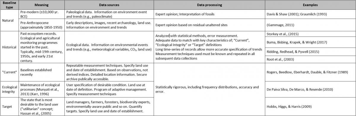
For example, the concept of “Zero Net Land Degradation” (Chasek et al., 2014) is clearly dependent on baselines for adaptive management and assessment of success. Multiple types of reference states are in use to furnish a start, baseline or reference condition for comparison with the current conditions (Table 4.2). A salutary warning of the danger of a lack of baseline was given by Alexander von Humboldt in 1848, as reported by Gritzner (1981), that travellers unfamiliar with arid lands are "easily led to adopt the erroneous inference that absence of trees is a characteristic of hot climates".

 

Target condition

 

Ecosystem services are provided to human beings and have no meaning apart from that. They are a measure of human preference and satisfaction, so a particularly pertinent reference condition for measurement of degradation would be one that maximizes the desired mix of ecosystem services – that is a Target condition. This is similar to the “utilitarian” concept of the Millennium Ecosystem Assessment (Hassan et al., 2005). A target condition is based on a deliberate choice and is therefore context dependent. For example, in the case of long-standing cropland agriculture, sustained and healthy crop production, rather than the natural land cover, is the target. This is perhaps the most important reference for policy purposes, since it represents a desired future state, the achievement of which can be measured and monitored. A target, however, is not static – it is an aim and aims can change, nor is it usually possible to treat a single service alone since any gain in one can cause a loss of another, so trade-offs are needed, and the choices involved can also change. Furthermore, in many regions and ecosystems, this potential is also not static because of ongoing regional and global changes such as climate change and atmospheric nitrogen deposition.

 

Historical baseline

 

The historical baseline is the condition of a site in the past. The change from the historical condition to the present time – the trend. This provides an objective assessment, as opposed to the selection of a Target condition which is an aspiration. A historical trend can indicate undesirable changes in an ecosystem and also point to the processes of degradation that have led to the current state and restoration efforts.

 

While highly desirable, unfortunately there are a few, detailed, time-series of observations of ecosystem properties that are more than 50 years old. Examples are the Park Grass Experiment started in 1856 (Silvertown et al., 2006) and selected plant communities throughout the Netherlands started in the 1930s (Smits et al., 2002). Most repetitive measurement programs are recent. Examples include the annual North American Breeding Bird Survey (Sauer et al., 2017); the many UK Biological Records Centre (Biological Records Centre, 2017) monitoring schemes; the 43-year Earth-Observing satellite record (Moran et al., 2012); and many “permanent plots” in which earlier surveys are repeated, often more than once (Bakker et al., 1996; Kapfer et al., 2017). Historical baselines have been used extensively for assessment of the status and trends of many species and ecosystems (e.g., the IUCN Red List of Threatened Species; IUCN, 2017). However, few of these records are coordinated, and start dates, repetitions and types of measurements generally differ, which makes comparisons difficult. Care must be taken to avoid a false impression of more or less degradation based on different starting points (Pauly, 1995). Furthermore, sites may have suffered degradation before the historical baseline (e.g. Gritzner, 1981).

 

Natural baseline In some circumstances, particularly where human influence and degradation are low, such as in isolated areas of boreal forest, remote humid forests and some islands, it may be reasonable to infer the condition before the first human influence from present land cover (Bull et al., 2014). This seems an obvious baseline from which to assess any trends in degradation and recovery, since it was before any human modification (Kotiaho et al., 2016), but practical and theoretical issues weigh against it. No exact date can be given for the first human occupation but it was sometime in the Holocene (≤10,000 BCE, but maybe only 2-300 years ago for some regions). Practically, it is rare to find objective data from so far into the past (Spikins, 2000). The only data of this type are fossil deposits, pollen and also fossil parts of plants, insects and diatoms and evidence of human-induced soil erosion that can provide some indications (Hoffmann et al., 2009). These can sometimes be dated or otherwise assigned to the pre-human period, but they are often too generalized to specify the state of the environment in adequate detail for comparison with existing conditions. Of course, a pre-human baseline has no use when the climate or other physical environmental conditions changed in the time between the baseline and the present time, for example the Little Ice Age just 400 years ago.

 

The start of the Anthropocene (approximately 1950) (Ludwig & Steffen, 2017; Morselli et al., 2018; Waters et al., 2016) can be a logical starting point for a natural baseline – an “Anthropocene baseline” – since it marks, by definition, the start of the massive acceleration of human influence on the natural environment and its biota. Data availability for the last 100 years is obviously more in number, type and accuracy. While anthropogenic degradation occurred in many places before the beginning of the Anthropocene, it was often negligible compared with the post-1950 period and is therefore a useful starting point to assess anthropogenic degradation.

 

However, even for an Anthropocene baseline, a significant amount of qualitative judgement is needed. One method is the “space for time” substitution (Johnson & Miyanishi, 2008; Pickett, 1989), which compares similar sites in different locations and treats spatial and temporal variation as equivalent. Although this assumption has been challenged, space-for-time substitution is often used due to necessity or convenience (Pickett, 1989). There is one respect in which the use of current conditions to infer a historical baseline is helpful, since non-anthropogenic, environmental changes, such as weather fluctuations will have affected both the supposed non-degraded sites and the putative degraded sites, thereby eliminating some non-anthropogenic environmental changes before the present time. A more objective method for inferring a former state from the current condition is by mathematical process modelling (McGrath et al., 2015; Spikins, 2000; Wang et al., 2006) but data are often sparse and spatial scales are coarse. There are many potential errors in modelling; for example, the mathematical representation of natural processes may not apply to the entire period between the current state and the original natural state.

 

 

Future trends of degradation

 

Accurate information on future environmental conditions and human effects on the environment would assist remediation and recovery efforts. Climate forecasting into an uncertain future needs to account for future land cover, changes in carbon sequestration and pollution. In order to have consistency in forecasts, “scenarios” have been developed that provide some descriptions of how the future might unfold. Scenarios are defined as “hypothetical sequences of events constructed for the purpose of focusing attention on causal processes and decision points” (Geist, 2005; Kahn & Wiener, 1967).

 

A range of plausible pathways, scenarios, and targets are used that capture a set of conditions for a range of land use, the efficiency of the use of land resources and products, trade and food self-sufficiency, effects of climate change, biodiversity, land use and so on. These are potential outcomes based on an internally consistent, reproducible, and plausible set of assumptions and theories of key driving forces of change (IPCC, 2000) but they should not be interpreted as forecasts.

 

Scenarios and their outcomes on climate change (Bjørnæs, 2015) use integrated assessment models that estimate the combined effects of human activities (e.g., land use and fossil fuel emissions) on the carbon-climate system. Integrated assessment models such as the IMAGE model (Integrated Model to Assess the Global Environment) (Stehfest et al., 2014) have been coupled with climate models (Moorcroft, 2003; Moss et al., 2010) to assess future environmental impacts (Meller et al., 2015) and livelihoods (Bos et al., 2015; IPCC, 2000) that simulate the interactions of human activities and climate. (2005-2100), providing a way to explore the implications of anthropogenic activities. 

 

References

 

Adeel, Z., Safriel, U., Niemeijer, D., & White, R. (2005). Millennium Ecosystem Assessment. Ecosystems and Human Well-being: Desertification Synthesis. Washington, D.C.: World Resources Institute.

Andreasen, J. K., O’Neill, R. V., Noss, R., & Slosser, N. C. (2001). Considerations for the development of a terrestrial index of ecological integrity. Ecological Indicators, 1(1), 21–35. https://doi.org/10.1016/S1470-160X(01)00007-3

August, P., Iverson, L., & Nugranad, J. (2002). Human Conversion of Terrestrial Habitats. In K. J. Gutzwiller (Ed.), Applying Landscape Ecology in Biological Conservation (pp. 198–224). Springer New York.

Bai, Z. G., Dent, D. L., Olsson, L., & Schaepman, M. E. (2008). Proxy global assessment of land degradation. Soil Use and Management, 24(3), 223–234. Retrieved from http://dx.doi.org/10.1111/j.1475-2743.2008.00169.x

Bakker, J. ., Olff, H., Willems, J. ., & Zobel, M. (1996). Why do we need permanent plots in the study of long-term vegetation dynamics? Journal of Vegetation Science, 7(2), 147–156. https://doi.org/10.2307/3236314

Baveye, P. c., & al.,  et. (2011). From Dust Bowl to Dust Bowl: Soils are Still Very Much a Frontier of Science. Soil Science Society of America, J., 75(6), 2037–2048. https://doi.org/doi:10.2136/sssaj2011.0145

Beinroth, F. H., Eswaran, H., & Reich, P. F. (2001). Global Assessment of Land Quality. (D. E. Stott, R. H. Mohtar, & G. C. Steinhardt, Eds.), Sustaining the Global Farm: Selected Papers from the 10th International Soil Conservation Organization Meeting. Purdue University and the USDA-ARS National Soil Erosion Research Laboratory. Retrieved from http://topsoil.nserl.purdue.edu/nserlweb-old/isco99/pdf/ISCOdisc/SustainingTheGlobalFarm/P233-Beinroth.pdf

Berry, L., Abraham, E., & Essahli, W. (2009). UNCCD recommended minimum set of impact indicators. UNCCD.

Biological Records Centre. (2017). Retrieved January 4, 2018, from https://www.ceh.ac.uk/our-science/projects/biological-records-centre

Bjørnæs, C. (2015). A guide to Representative Concentration Pathways. Oslo. Retrieved from https://www.sei-international.org/mediamanager/documents/A-guide-to-RCPs.pdf

Bos, S. P. M., Pagella, T., Kindt, R., Russell, A. J. M., & Luedeling, E. (2015). Climate analogs for agricultural impact projection and adaptation—a reliability test. Frontiers in Environmental Science, 3. https://doi.org/10.3389/fenvs.2015.00065

Brown, E. D., & Williams, B. K. (2016). Ecological integrity assessment as a metric of biodiversity: are we measuring what we say we are? Biodiversity Conservation, 25, 1011–1035. https://doi.org/10.1007/s10531-016-1111-0

Brus, D., Tomislav, H., Bas, K., Mulder, T. I., Poggio, L., Ribeiro, E., & Omuto, C. T. (2017). SOIL ORGANIC CARBON MAPPING Cookbook. (R. R. V. Yusuf Yigini, Rainer Baritz, Ed.) (2nd ed.). Rome, Italy: FOOD AND AGRICULTURE ORGANIZATION OF THE UNITED NATIONS. Retrieved from http://www.fao.org/3/a-bs901e.pdf

Bull, J. W., Gordon, A., Law, E. A., Suttle, K. B., & Milner-Gulland, E. J. (2014). Importance of Baseline Specification in Evaluating Conservation Interventions and Achieving No Net Loss of Biodiversity. Conservation Biology, 28(3), 799–809. https://doi.org/10.1111/cobi.12243

Buma, B., Bisbing, S., Krapek, J., & Wright, G. (2017). A foundation of ecology rediscovered: 100 years of succession on the William S. Cooper plots in Glacier Bay, Alaska. Ecology, 98(6), 1513–1523. https://doi.org/10.1002/ecy.1848

Cai, X., Zhang, X., & Wang, D. (2011). Land Availability for Biofuel Production. Environmental Science & Technology, 45(1), 334–339. https://doi.org/10.1021/es103338e

Campbell, J. E., Lobell, D. B., Genova, R. C., & Field, C. B. (2008). The Global Potential of Bioenergy on Abandoned Agriculture Lands. Environmental Science & Technology, 42(15), 5791–5794. https://doi.org/10.1021/es800052w

Castro, J. M., Salomone, J. M., & Reichart, R. N. (1980). Estudio de los focos de erosión en el SO de la Provincia de Chubut. Informe Técnico (Vol. 15). Trelew, Argentina: Instituto Nacional de Tecnología Agropecuaria:

Chasek, P., Safriel, U., Shikongo, S., & Fuhrman, V. F. (2014). Operationalizing Zero Net Land Degradation: The next stage in international efforts to combat desertification? Journal of Arid Environments, (0). https://doi.org/http://dx.doi.org/10.1016/j.jaridenv.2014.05.020

Cherlet, M., Ivits, E., Kutnjak, H., Smid, M., Sommer, S., & Zucca, C. (2015). The World Atlas of Desertification assessment concept for conscious land use solutions. Geophysical Research Abstracts EGU General Assembly, 17, 2015–15871. Retrieved from http://meetingorganizer.copernicus.org/EGU2015/EGU2015-15871.pdf

Convention on Biological Diversity. (2016). Framework and Guiding Principles for a Land Degradation Indicator: Outcomes of the Expert Meeting. Wahington D.C.

Creswell, J. W. (2007). Designing and conducting mixed methods . Thousand Oaks. Thousand Oaks, CA: Sage Publications.

Davis, M. B., & Shaw, R. G. (2001). Range shifts and adaptive responses to Quaternary climate change. Science (New York, N.Y.), 292(5517), 673–679. https://doi.org/10.1126/science.292.5517.673

De Paiva Silva, D., De Marco, P., & Resende, D. C. (2010). Adult odonate abundance and community assemblage measures as indicators of stream ecological integrity: A case study. Ecological Indicators, 10, 744–752. https://doi.org/doi:10.1016/j.ecolind.2009.12.004

Dregne, H. E., & Chou, N. T. (1992). Global desertification dimensions and costs. In H. E. Dregne (Ed.), Degradation & restoration of arid lands. Lubbock, Texas: International Center for Arid and Semiarid Land Studies, Texas Tech. University.

Ellis, E. C., Goldewijk, K. K., Siebert, S., Lightman, D., & Ramankutty, N. (2010). Anthropogenic transformation of the biomes, 1700 to 2000. Global Ecology and Biogeography, 19(5), 589–606. https://doi.org/10.1111/j.1466-8238.2010.00540.x

Ellis, E. C., & Ramankutty, N. (2008). Putting people in the map: anthropogenic biomes of the world. Frontiers in Ecology and the Environment, 6(8), 439–447. https://doi.org/doi: 10.1890/070062

Eswaran, H., Lal, R., & Reich, P. F. (2001). Land degradation: an overview. (E. M. Bridges, I. D. Hannam, L. R. Oldeman, F. W. T. Pening de Vries, S. J. Scherr, & S. Sompatpanit, Eds.), Responses to Land Degradation. Khon Kaen, Thailand: Oxford Press, New Delhi, India.

Eswaran, H., & Reich, P. (1998). Desertification: a global assessment and risks to sustainability. In Proceedings of the 16th International Congress of Soil Science. Montpellier, France.

FAO. (2001). Food and Agriculture Organization Global Forest resources assessment 2000: FAO Forestry Paper 140. Rome.

FAO. (2002). Terrastat: Global land resources GIS models and databases for poverty and food insecurity mapping. Rome, Italy: Food and Agriculture Organization FAO - NRLA. Retrieved from http://www.fao.org/geonetwork/srv/en/main.home

Forman, R. T. T. (1995). Some general principles of landscape and regional ecology. Landscape Ecology, 10(3), 133–142. https://doi.org/10.1007/BF00133027

Gammage, B. (2011). The biggest estate on earth : how Aborigines made Australia. Allen & Unwin. Retrieved from http://trove.nla.gov.au/work/154959343?q&versionId=185191842

Geist, H. (2005a). The Causes and Progression of Desertification. Ashgate Studies in Environmental Policy and Practice. Abingdon Oxon, UK: Ashgate Publishing. https://doi.org/10.1177/0309133306071155

Geist, H. (2005b). The Causes and Progression of Desertification. Ashgate Studies in Environmental Policy and Practice. Abingdon Oxon, UK: Ashgate Publishing. https://doi.org/10.1177/0309133306071155

Gholizadeh, H., Gamon, J. A., Zygielbaum, A. I., Wang, R., Schweiger, A. K., & Cavender-Bares, J. (2018). Remote sensing of biodiversity: Soil correction and data dimension reduction methods improve assessment of α-diversity (species richness) in prairie ecosystems. Remote Sensing of Environment, 206, 240–253. https://doi.org/10.1016/j.rse.2017.12.014

Gibbs, H. K., & Salmon, J. M. (2015). Mapping the world’s degraded lands. Applied Geography, 57, 12–21. https://doi.org/http://dx.doi.org/10.1016/j.apgeog.2014.11.024

Graumlich, L. A. (1993). A 1000-Year Record of Temperature and Precipitation in the Sierra Nevada. Quaternary Research, 39(2), 249–255. https://doi.org/10.1006/QRES.1993.1029

Gritzner, J. A. (1981). Environmental degradation in Mauritania. Wahington, D.C.: National Academy Press.

Hassan, R., Scholes, R., & Ash, N. (Eds.). (2005). Millennium Ecosystem Assessment: Ecosystems and Human Well-Being. Washington, D.C.: Island Press.

Herrmann, S. M., & Sop, T. K. (2016). The Map Is not the Territory: How Satellite Remote Sensing and Ground Evidence Have Re-shaped the Image of Sahelian Desertification. In R. Behnke & M. Mortimore (Eds.), The End of Desertification? : Disputing Environmental Change in the Drylands (pp. 117–145). Berlin, Heidelberg: Springer Berlin Heidelberg. https://doi.org/10.1007/978-3-642-16014-1_5

Hobbs, R. J., Higgs, H., & Harris, J. A. (2009). Novel ecosystems: implications for conservation and restoration. Trends in Ecology & Evolution, 24(11), 599–605. https://doi.org/10.1016/J.TREE.2009.05.012

Hoffmann, T., Erkens, G., Gerlach, R., & Klostermann, J. (2009). Trends and controls of Holocene floodplain sedimentation in the Rhine catchment. CATENA, 77(2), 96–106. https://doi.org/10.1016/j.catena.2008.09.002

Hurt, R. D. (1986). Federal Land Reclamation in the Dust Bowl. Great Plains Quarterly, 968, 106. Retrieved from http://digitalcommons.unl.edu/greatplainsquarterly/968

Ibáñez, J., Valderrama, J. M., Puigdefábregas, J., Martínez Valderrama, J., & Puigdefabregas, J. (2008). Assessing desertification risk using system stability condition analysis. Ecological Modelling, 213(2), 180–190. https://doi.org/doi:10.1016/j.ecolmodel.2007.11.017

IPCC. (2000). IPCC Special Report Emissions Scenarios. Summary for Policymakers Emissions Scenarios. Retrieved from https://ipcc.ch/pdf/special-reports/spm/sres-en.pdf

IUCN. (2017). The IUCN Red List of Threatened Species. Retrieved October 11, 2017, from http://www.iucnredlist.org

Izaurralde, R. C., Williams, J. R., Post, W. M., Thomson, A. M., McGill, W. B., Owens, L. B., & Lal, R. (2007). Long-term modeling of soil C erosion and sequestration at the small watershed scale. Climatic Change, 80(1–2), 73–90. https://doi.org/10.1007/s10584-006-9167-6

Jackson, H., & Prince, S. D. (2016). Degradation of net primary production in a semiarid rangeland. Biogeosciences, 13(16), 4721–4734. https://doi.org/10.5194/bg-13-4721-2016

Jeltsch, F., Milton, S. J., Dean, W. R. J., & Van Rooyen, N. (1997). Analysing Shrub Encroachment in the Southern Kalahari: A Grid-Based Modelling Approach. Journal of Applied Ecology, 34(6), 1497–1508. https://doi.org/10.2307/2405265

Johnson, E. A., & Miyanishi, K. (2008). Testing the assumptions of chronosequences in succession. Ecology Letters, 11(5), 419–431. https://doi.org/10.1111/j.1461-0248.2008.01173.x

Kahn, H., & Wiener, J. A. (1967). The Year 2000: A Framework for Speculation on the Next Thirty-three Years. New York, USA: Macmillan.

Kapfer, J., Hédl, R., Jurasinski, G., Kopecký, M., Schei, F. H., & Grytnes, J.-A. (2017). Resurveying historical vegetation data - opportunities and challenges. Applied Vegetation Science, 20(2), 164–171. https://doi.org/10.1111/avsc.12269

Karr, J. R. (1991). Biological Integrity: A Long-Neglected Aspect of Water Resource Management. Ecological Applications, 1(1), 66–84. https://doi.org/10.2307/1941848

Karr, J. R. (1996). Ecological integrity and ecological health are not the same. In P. Schultz (Ed.), Engineering Within Ecological Constraints (pp. 97–110). Washington D.C.: National Academy of Engineering.

Kirkby, M. J., Irvine, B. J., Jones, R. J. A., & Govers, G. (2008). The PESERA coarse scale erosion model for Europe. I. – Model rationale and implementation. European Journal of Soil Science, 59(6), 1293–1306. https://doi.org/10.1111/j.1365-2389.2008.01072.x

Kosmas, C., Karavitis, C., Kairis, O., Kounalaki, A., Fasouli, V., & Tsesmelis, D. (2012). Using indicators for identifying best land management practices for combating desertification. DESIRE Scientific reports. Deliverable 2.2.3. Agricultural University of Athens.

Kotiaho, J. S., ten Brink, B., & Harris, J. (2016). Land use: A global baseline for ecosystem recovery. Nature, 532(7597), 37–37. https://doi.org/10.1038/532037c

Lambin, E. F., & Geist, H. J. (2008). Land-use and land-cover change: local processes and global impacts. Berlin: Springer.

Liniger, H., Schwilch, G., Gurtner, M., Studer, R. M., Hauert, C., van Lynden, G., & Critchley, W. (2008). WOCAT Degradation Categorization System. WOCAT - World Overview of Conservation Approaches and Technologies. Retrieved from https://www.wocat.net/fileadmin/user_upload/documents/QT_and_QA/CategorisationSystem.pdf

Lockwood, J., & Lockwood, D. (1993). Catastrophe Theory: A Unified Paradigm for Rangeland Ecosystem Dynamics. Journal of Range Management, 46(4), 282–288. https://doi.org/http10.2307/4002459

Lorenz, K., & Lal, R. (2016). Soil Organic Carbon – An Appropriate Indicator to Monitor Trends of Land and Soil Degradation within the SDG Framework? (S. M. Starke & K. Ehlers, Eds.). Retrieved from http://www.umweltbundesamt.de/publikationen

Ludwig, C., & Steffen, W. (2017). The 1950s as the Beginning of the Anthropocene. In Reference Module in Earth Systems and Environmental Sciences. Elsevier. https://doi.org/10.1016/B978-0-12-409548-9.09940-1

McGrath, M. J., Luyssaert, S., Meyfroidt, P., Kaplan, J. O., Buergi, M., Chen, Y., Erb, K., Gimmi, U., McInerney, D., Naudts, K., Otto, J., Pasztor, F., Ryder, J., Schelhaas, M.-J., & Valade, A. (2015). Reconstructing European forest management from 1600 to 2010. BIOGEOSCIENCES, 12(14), 4291–4316. https://doi.org/10.5194/bg-12-4291-2015

McRae, L., Deinet, S., & Freeman, R. (2017). The Diversity-Weighted Living Planet Index: Controlling for Taxonomic Bias in a Global Biodiversity Indicator. PLOS ONE, 12(1), e0169156. https://doi.org/10.1371/journal.pone.0169156

Meller, L., van Vuuren, D. P., & Cabeza, M. (2015). Quantifying biodiversity impacts of climate change and bioenergy: the role of integrated global scenarios. Regional Environmental Change, 15(6), 961–971. https://doi.org/10.1007/s10113-013-0504-9

Millennium Ecosystem Assessment. (2005). Ecosystems and Human Well-being, vol 1. Current State and Trends: Findings of the Condition and Trends Working Millennium Chapter 22,. In Ecosystem Assessment Series. Dryland Systems, Chapter 22 (p. p 815).

Milton, S. J., Dean, W. R. J., du Plessis, M., & Siegfried, W. R. (1994). A conceptual model of arid rangeland degradation. Bioscience, 44(2), 70–76. https://doi.org/10.2307/1312204

Moorcroft, P. R. (2003). Recent advances in ecosystem-atmosphere interactions: an ecological perspective. Proceedings of the Royal Society B-Biological Sciences, 270(1521), 1215–1227.

Moran, E. F., Skole, D. L., & Turner, B. L. (2012). The Development of the International Land-Use and Land-Cover Change (LUCC) Research Program and Its Links to NASA’s Land-Cover and Land-Use Change (LCLUC) Initiative. In G. Gutman, A. C. Janetos, C. O. Justice, E. F. Moran, J. F. Mustard, R. R. Rindfuss, D. Skole, B. L. TurnerII, & M. A. Cochrane (Eds.), Land Change Science - Observing, Monitoring and Understanding Trajectories of Change on the Earth’s Surface (pp. 1–15). Dordrecht: Springer, Dordrecht. https://doi.org/10.1007/978-1-4020-2562-4_1

Morselli, M., Vitale, C. M., Ippolito, A., Villa, S., Giacchini, R., Vighi, M., & Di Guardo, A. (2018). Predicting pesticide fate in small cultivated mountain watersheds using the DynAPlus model: Toward improved assessment of peak exposure. Science of The Total Environment, 615, 307–318. https://doi.org/10.1016/j.scitotenv.2017.09.287

Moss, R. H., Edmonds, J. A., Hibbard, K. A., Manning, M. R., Rose, S. K., van Vuuren, D. P., Carter, T. R., Emori, S., Kainuma, M., Kram, T., Meehl, G. A., Mitchell, J. F. B., Nakicenovic, N., Riahi, K., Smith, S. J., Stouffer, R. J., Thomson, A. M., Weyant, J. P., & Wilbanks, T. J. (2010). The next generation of scenarios for climate change research and assessment. Nature, 463(7282), 747–756. https://doi.org/10.1038/nature08823

Munyati, C., Economon, E. B., & Malahlela, O. E. (2013). Effect of canopy cover and canopy background variables on spectral profiles of savanna rangeland bush encroachment species based on selected Acacia species (mellifera, tortilis, karroo) and Dichrostachys cinerea at Mokopane, South Africa. Journal of Arid Environments, 94(0), 121–126. https://doi.org/http://dx.doi.org/10.1016/j.jaridenv.2013.02.010

Nachtergaele, F. O. F., & Licona-Manzur, C. (2008). The Land Degradation Assessment in Drylands (LADA) Project: Reflections on Indicators for Land Degradation Assessment. In C. C. Lee & T. Schaaf (Eds.), The Future of Drylands (pp. 327–348). Food and Agriculture Organization of the United Nations (FAO), Rome, Italy: UNESCO.

National Research Council. (2000). Ecological Indicators for the Nation. Washington, D.C.: National Academies Press. https://doi.org/10.17226/9720

Noojipady, P., Prince, S. D., & Rishmawi, K. (2015). Reductions in productivity due to land degradation in the drylands of the southwestern United States. Ecosystem Health and Sustainability, 1(8), art27. https://doi.org/10.1890/EHS15-0020.1

Oldeman, L. R., Hakkeling, R. T. A., & Sombroek, W. G. (1991). World map of the status of human-induced soil degradation: an explanatory note. Global Assessment of Soil Degradation (GLASOD) (2nd ed.). Wageningen: Winand Staring Center, International Society for Soil Science, FAO, International Institute for Aerospace Survey and Earth Science.

Olsson, L., Eklundh, L., & Ardö, J. (2005). A recent greening of the Sahel—trends, patterns and potential causes. Journal of Arid Environments, 63(3), 556–566. https://doi.org/10.1016/j.jaridenv.2005.03.008

Pauly, D. (1995). Anecdotes and the shifting baseline syndrome of fisheries. Trends in Ecology and Evolution, 10(10), 430.

Petchel-Held, G., Block, A., & Cassel-Gintz. (1999). Syndromes of global change:a qualitative modelling approachto assist global environmental management. ENVIRONMENTAL MODELING and  ASSESSMENT, 4, 295–314.

Peters, D. P. C., Lauenroth, W. K., & Burke, I. C. (2008). The role of disturbance in community and ecosystem dynamics. In W. K. Lauenroth & I. C. Burke (Eds.), Ecology of the short grass steppes: a long-term perspective (pp. 84–118). Oxford, UK: Oxford University Press.

Pickett, S. T. A. (1989). Space-for-Time Substitution as an Alternative to Long-Term Studies. In G. E. Likens (Ed.), Long-Term Studies in Ecology: Approaches and Alternatives (pp. 110–135). New York, NY: Springer New York. https://doi.org/10.1007/978-1-4615-7358-6_5

Pratt, C. R., Kaly, U. L., & Mitchell, J. (2004). Manual: How to Use the Environmental Vulnerability Index (EVI).

Prince, S. D. (1991). A model of regional primary production for use with coarse-resolution satellite data. International Journal of Remote Sensing, 12(6), 1313–1330.

Prince, S. D. (2016). Where does desertification occur? Mapping dryland degradation at regional to global scales. In R. Behnke & M. Mortimore (Eds.), In The End of Desertification? Disputing Environmental Change in the Drylands. Springer‐Praxis Earth System Science Series.

Prince, S. D., Becker-Reshef, I., & Rishmawi, K. (2009). Detection and mapping of long-term land degradation using local net production scaling: Application to Zimbabwe. Remote Sensing of Environment, 113(5). https://doi.org/10.1016/j.rse.2009.01.016

Prince, S. D., De Colstoun, E. B., & Kravitz, L. L. (1998). Evidence from rain-use efficiencies does not indicate extensive Sahelian desertification. Global Change Biology, 4(4), 359–374. https://doi.org/10.1046/j.1365-2486.1998.00158.

Ridding, L. E., Redhead, J. W., & Pywell, R. F. (2015). Fate of semi-natural grassland in England between 1960 and 2013: A test of national conservation policy. Global Ecology and Conservation, 4, 516–525. https://doi.org/10.1016/j.gecco.2015.10.004

Rishmawi, K., Prince, S., & Xue, Y. (2016). Vegetation Responses to Climate Variability in the Northern Arid to Sub-Humid Zones of Sub-Saharan Africa. Remote Sensing, 8(11), 910. https://doi.org/10.3390/rs8110910

Robbins, P. (2012). Political ecology : a critical introduction (2nd editio). Chichester, U.K.: John Wiley.

Rogers, L. E., Beedlow, P. A., Eberhardt, L. E., Dauble, D. D., & Fitzner, R. E. (1989). Ecological baseline study of the Yakima Firing Center proposed land acquisition: A status report. Richland, WA (United States). https://doi.org/10.2172/6519080

Romm, J. (2011). The next dustbowl. Nature, 478, 450–451.

Root, T. L., Price, J. T., Hall, K. R., Schneider, S. H., Rosenzweig, C., & Pounds, J. A. (2003). Fingerprints of global warming on wild animals and plants. Nature, 421(6918), 57–60. https://doi.org/10.1038/nature01333

Safriel, U. (2009). Deserts and desertification: Challenges but also opportunities. Land Degradation & Development, 20(4), 353–366. https://doi.org/10.1002/ldr.935

Sauer, J., Niven, D., Hines, J., Ziolkowski, D., Pardieck, K. L., Fallon, J. E., & Link, W. (2017). The North American Breeding Bird Survey, results and analysis 1966 - 2015. https://doi.org/10.5066/F7C24TNP

Sietz, D., Untied, B., Walkenhorst, O., Ludeke, M. K. B., Mertins, G., Petschel-Held, G., & Schellnhuber, H. J. (2006). Smallholder agriculture in Northeast Brazil: assessing heterogeneous human-environmental dynamics. Regional Environmental Change, 6(3), 132–146.

Silvertown, J., Poulton, P., Johnston, E., Edwards, G., Heard, M., & Biss, P. M. (2006). The Park Grass Experiment 1856-2006: its contribution to ecology. Journal of Ecology, 94(4), 801–814. https://doi.org/10.1111/j.1365-2745.2006.01145.x

Smits, N. A. C., Schaminée, J. H. J., & van Duuren, L. (2002). 70 years of permanent plot research in The Netherlands. Applied Vegetation Science, 5(1), 121–126. https://doi.org/10.1658/1402-2001(2002)005[0121:YOPPRI]2.0.CO;2

Sonneveld, B. G., & Dent, D. L. (2009). How good is GLASOD? Journal of Environmental Management, 90(1), 274–283. https://doi.org/10.1016/j.jenvman.2007.09.008

Spikins, P. (2000). GIS Models of Past Vegetation: An Example from Northern England, 10,000–5000BP. Journal of Archaeological Science, 27(3), 219–234. https://doi.org/10.1006/jasc.1999.0449

Steffen, W., Leinfelder, R., Zalasiewicz, J., Waters, C. N., Williams, M., Summerhayes, C., Barnosky, A. D., Cearreta, A., Crutzen, P., Edgeworth, M., Ellis, E. C., Fairchild, I. J., Galuszka, A., Grinevald, J., Haywood, A., Ivar do Sul, J., Jeandel, C., McNeill, J. R., Odada, E., Oreskes, N., Revkin, A., Richter, D. deB., Syvitski, J., Vidas, D., Wagreich, M., Wing, S. L., Wolfe, A. P., & Schellnhuber, H. J. (2016). Stratigraphic and Earth System approaches to defining the Anthropocene. Earth’s Future. https://doi.org/10.1002/2016EF000379

Steffen, W., Richardson, K., Rockström, J., Cornell, S. E., Fetzer, I., Elena M. B., Biggs, R., Carpenter, S. R., de Vries, W., de Wit, C. A., Folke, C., Gerten, D., Heinke, J., Mace, G. M., Persson, L. M., Ramanathan, V., Reyers, B., & Sörlin, S. (2015). Planetary boundaries: Guiding human development on a changing planet. Science, 347(6223, 1259855). https://doi.org/10.1126/science.1259855

Stehfest, E., van Vuuren, D., Kram, T., Bouwman, L., Alkemade, R., Bakkenes, M., Biemans, H., Bouwman, A., den Elzen, M., Janse, J., Lucas, P., van Minnen, J., Müller, M., & Prins, A. (2014). Integrated Assessment of Global Environmental Change with IMAGE 3.0. Model description and policy applications. (L. B. Elke Stehfest, Detlef van Vuuren, Tom Kram, Ed.). The Hague: PBL Netherlands Environmental Assessment Agency.

Storkey, J., Macdonald, A. J., Poulton, P. R., Scott, T., Köhler, I. H., Schnyder, H., Goulding, K. W. T., & Crawley, M. J. (2015). Grassland biodiversity bounces back from long-term nitrogen addition. Nature, 528(7582), 401–404. https://doi.org/10.1038/nature16444

Symeonakis, E., & Drake, N. (2004). Monitoring desertification and land degradation over sub-Saharan Africa. International Journal of Remote Sensing, 25(3), 573–592. Retrieved from http://sfx.umd.edu:9003/cp?&atitle=Monitoring+desertification+and+land+degradation+over+sub-Saharan+Africa&auinit=E&aulast=Symeonakis&date=2004&epage=592&issn=0143-1161&issue=3&sid=ISI:WoK&spage=573&stitle=INT+J+REMOTE+SENS&title=INTERNATIONAL+JOURNAL+OF+

Tamene, L., & Le, Q. B. (2015). Estimating soil erosion in sub-Saharan Africa based on landscape similarity mapping and using the revised universal soil loss equation (RUSLE). Nutrient Cycling in Agroecosystems, 101, 1–15, NaN-15-9674–9679. https://doi.org/10.1007/s10705-015-9674-9

The Nature Conservancy. (2016). When the dust settled. U.S. Farm Bill Conservation Programs Have Roots in Dirty Thirties. Retrieved March 19, 2017, from https://www.nature.org/ourinitiatives/regions/northamerica/when-the-dust-settled.xml

Thomas, D. S. G., & Middleton, N. J. (1994). Desertification: exploding the myth. Chichester: John Wiley.

Tucker, C.J., Pinzon, J. (2016). Using spectral vegetation indices to measure gross primary productivity as an indicator of land degradation. Washington, D.C.

Tucker, C. J., Dregne, H. E., & Newcomb, W. W. (1991). Expansion and contraction of the Sahara desert from 1980 to 1990. Science, 253, 299–301.

Turnbull, L., Wainwright, J., & Brazier, R. E. (2008). A conceptual framework for understanding semi-arid land degradation: ecohydrological interactions across multiple-space and time scales. Ecohydrology, 1(1), 23–34. https://doi.org/10.1002/eco.4

Turner, B. L., Meyer, W. B., & Skole, D. L. (1994). Global land-use land-cover change - towards an integrated study. Ambio, 23(1), 91–95. https://doi.org/10.2307/4314168

UNCCD. (2017). The Global Land Outlook. Retrieved July 14, 2017, from http://knowledge.unccd.int/knowledge-products-and-pillars/access-capacity-policy-support-technology-tools/global-land-outlook

UNEP. (1997). World Atlas of Desertification (2nd ed.). London & New York: Arnold & Wiley, on behalf of UNEP.

United Nations. (2015). Transforming our world: the 2030 Agenda for Sustainable Development .:. Sustainable Development Knowledge Platform. Retrieved February 23, 2018, from https://sustainabledevelopment.un.org/post2015/transformingourworld

Vagen, T. G., Lal, R., & Singh, B. R. (2005). Soil carbon sequestration in sub-Saharan Africa: A review. Land Degradation & Development, 16(1), 53–71.

Vitousek, P. M., Mooney, H. A., Lubchenco, J., & Melillo, J. M. (1997). Human domination of Earth’s ecosystems. Science, 277(494), 499.

Vogt, J. V, Safriel, U., Von Maltitz, G., Sokona, Y., Zougmore, R., Bastin, G., & Hill, J. (2011). Monitoring and assessment of land degradation and desertification: Towards new conceptual and integrated approaches. Land Degradation & Development, 22(2), 150–165. https://doi.org/10.1002/ldr.1075

Wang, A., Price, D. T., & Arora, V. (2006). Estimating changes in global vegetation cover (1850-2100) for use in climate models. Global Biogeochemical Cycles, 20(3), n/a-n/a. https://doi.org/10.1029/2005GB002514

Waters, C. N., Zalasiewicz, J., Summerhayes, C., Barnosky, A. D., Poirier, C., Gałuszka, A., Cearreta, A., Edgeworth, M., Ellis, E. . C., Ellis, M., Jeandel, C., Leinfelder, R., McNeill, J. . R., Richter, D. deB., Steffen, W. L., Syvitski, J., Vidas, D., Wagreich, M., Williams, M., Zhisheng, A., Grinevald, J., Odada, E., Oreskes, N., & Wolfe, A. . P. (2016). The Anthropocene is functionally and stratigraphically distinct from the Holocene. Science, 351(6269). https://doi.org/10.1126/science.aad2622

Webb, R. H. (2002). Recovery of Severely Compacted Soils in the Mojave Desert, California, USA. Arid Land Research and Management , 16, 291–305. https://doi.org/: 10.1080=15324980290000403

Weber, G. E., Moloney, K., & Jeltsch, F. (2000). Simulated long-term vegetation response to alternative stocking strategies in savanna rangelands. Plant Ecology, 150(1/2), 77–96. https://doi.org/10.1023/A:1026570218977

Wessels, K. J., Prince, S. D., Carroll, M., & Malherbe, J. (2007). Relevance of rangeland degradation in semiarid northeastern South Africa to the nonequilibrium theory. Ecological Applications, 17(3), 815–827.

Wessels, K. J., Prince, S. D., & Reshef, I. (2008). Mapping land degradation by comparison of vegetation production to spatially derived estimates of potential production. Journal of Arid Environments, 72(10). https://doi.org/10.1016/j.jaridenv.2008.05.011

Wessels, K. J., van den Bergh, F., & Scholes, R. J. (2012). Limits to detectability of land degradation by trend analysis of vegetation index data. Remote Sensing of Environment, 125(0), 10–22. https://doi.org/10.1016/j.rse.2012.06.022

Wiegand, K., Saitz, D., & Ward, D. (2006). A patch-dynamics approach to savanna dynamics and woody plant encroachment - Insights from an arid savanna. Perspectives in Plant Ecology Evolution and Systematics, 7(4), 229–242. https://doi.org/10.1016/j.ppees.2005.10.001

Wiegand, T., & Milton, S. J. (1996). Vegetation change in semi arid communities. Vegetatio, 125, 169–183. Retrieved from https://link.springer.com/content/pdf/10.1007/BF00044649.pdf

Wiegand, T., Milton, S. J., & Wissel, C. (1995). A Simulation Model for Shrub Ecosystem in the Semiarid Karoo, South Africa. Ecology, 76(7), 2205–2221. https://doi.org/10.2307/1941694

World Wildlife Fund. (2016). Living Planet Report 2016 : Risk and resilience in a new ear. Gland, Switzerland: WWF International.

Zucca, C., & Biancalani, R. (2011). Guidelines for the use of the LADA QM DB in the frame of the “National Piloting of provisional UNCCD impact indicators” (Version 3). LADA FAO.